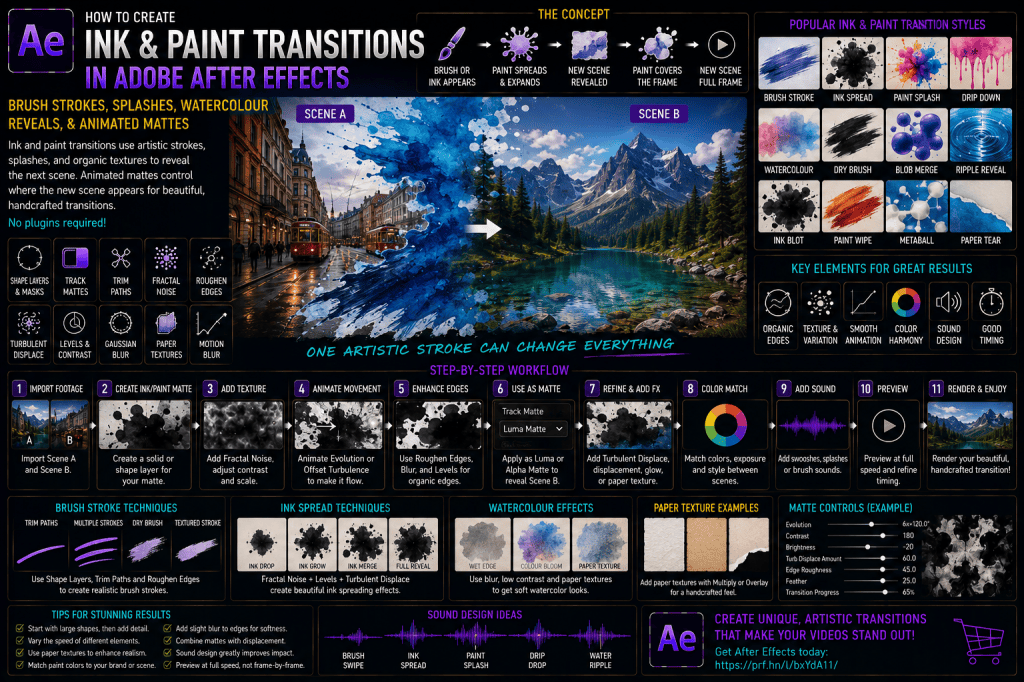
A digital scan transition makes a scene appear as though it is being detected, analyzed, generated, or reconstructed by a machine.

Instead of using a conventional wipe, the next image is revealed progressively by:

• scanning lines;
• laser sweeps;
• digital grids;
• holographic bands;
• data particles;
• glowing edges;
• signal noise;
• pixel reconstruction;
• HUD overlays.

The result can feel like a futuristic imaging system, AI scanner, security interface, holographic display, or digital mapping device.

The basic structure is:

Scene A → scan begins → image breaks into digital information → scanning line crosses frame → Scene B reconstructs → interface stabilizes

In Adobe After Effects, this effect can be created using native tools such as:

• Shape Layers;
• Track Mattes;
• Gradient Ramp;
• Fractal Noise;
• Displacement Map;
• Glow;
• Venetian Blinds;
• Grid;
• Find Edges;
• Tint;
• Noise;
• CC Ball Action;
• masks;
• expressions;
• Motion Blur.

This tutorial covers several scan styles, from a simple horizontal sweep to a complete holographic reconstruction transition.

Affiliate disclosure: This article contains affiliate links. If you purchase Adobe After Effects through one of these links, we may earn a commission at no additional cost to you.

What Is a Digital Scan Transition?

A digital scan transition creates the illusion that an image is being progressively read or reconstructed.

Imagine a bright horizontal line moving downward across a city.

Above the line:

Scene A remains visible.

Below the line:

Scene B has already been generated.

The moving boundary might contain:

Glow.

pixel noise.

data particles.

digital distortion.

outline highlights.

That single moving line becomes the visual mechanism of the transition.

Digital scan transitions are especially useful for:

technology videos.

AI content.

cybersecurity.

mapping.

gaming.

product demonstrations.

science visuals.

HUD interfaces.

futuristic presentations.

motion graphics.

If you’d like to build these effects yourself, you can explore Adobe’s current After Effects options here:

Explore Adobe After Effects and current plans

The Core Scan Concept

Most scan transitions use three main layers:

SCENE_A

SCAN_MATTE

SCENE_B

The scan matte determines where Scene B becomes visible.

For example:

top half black.

bottom half white.

Move the boundary downward.

Scene B is progressively revealed.

The transition becomes much more convincing once that boundary is enhanced with:

Glow.

noise.

distortion.

grids.

particles.

Project 1 — Basic Horizontal Scan

Let’s create the simplest version first.

Step 1: Create the Composition

Create:

DIGITAL_SCAN_MASTER

Suggested settings:

1920 × 1080.

30 fps.

10 seconds.

Import:

SCENE_A

and:

SCENE_B

Place Scene B above Scene A.

Step 2: Create the Scan Matte

Create:

Layer → New → Solid

Rename:

SCAN_MATTE

Step 3: Add a Rectangular Mask

Draw a large rectangle covering the lower portion of the frame.

Scene B will eventually be revealed through this shape.

Step 4: Animate Mask Position

Start with the mask below the composition.

Move it upward or downward depending on the desired scan direction.

For this example:

start at top.

move toward bottom.

Step 5: Use as Track Matte

Use SCAN_MATTE as:

Alpha Matte

for Scene B.

Now Scene B appears progressively behind the moving boundary.

Project Result

Scene A visible.

Boundary moves downward.

Scene B appears behind it.

Scene B fills the frame.

That is the most basic digital scan transition.

PART 2 — ADD THE SCANNING LINE

The transition needs a visible scanning edge.

Step 6: Create Shape Layer

Create:

SCAN_LINE

Draw a horizontal line.

Step 7: Add Stroke

Use:

bright cyan.

white.

green.

or another digital color.

Step 8: Add Glow

Apply:

Glow.

Increase:

Glow Radius.

Glow Intensity.

Step 9: Parent to Scan Matte

Animate SCAN_LINE so it remains exactly on the boundary between Scene A and Scene B.

Project 2 — Laser Scan Reveal

Scene A.

bright scanning line travels downward.

Scene B becomes visible behind it.

Glow leaves a subtle trailing effect.

PART 3 — SCAN LINE THICKNESS

A thin scan line feels technical.

A thicker band feels more like a holographic reconstruction beam.

Try:

2 px.

5 px.

20 px.

50 px.

PART 4 — MULTI-LINE SCANNER

Instead of one line:

create several parallel lines.

For example:

main bright line.

two dimmer trailing lines.

one noisy leading line.

This creates more visual complexity.

PART 5 — TRAILING GLOW

Duplicate SCAN_LINE.

Blur heavily.

Reduce Opacity.

Offset slightly behind.

The scan now leaves a temporary glowing trail.

Project 3 — Enhanced Scan Beam

Bright line.

soft glow.

thin secondary lines.

slight noise.

Scene B appears beneath.

PART 6 — VERTICAL SCAN

Rotate the entire concept 90°.

Move:

left → right.

or:

right → left.

This works particularly well for:

portraits.

products.

interface panels.

PART 7 — DIAGONAL SCAN

Create a diagonal rectangular matte.

Move:

bottom-left → top-right.

Add matching diagonal scan line.

PART 8 — RADIAL SCAN

Scanning doesn’t need to be linear.

Create:

circular matte.

Animate Scale.

Scene B appears from center outward.

Add a circular glowing edge.

Project 4 — Radar-Style Reveal

Small circle appears.

expands.

Scene B becomes visible inside.

ring glows.

Scene B fills frame.

PART 9 — RADAR SWEEP

Create a rotating wedge rather than expanding circle.

Use Shape Layer:

pie-shaped sector.

Rotate around center.

Scene B appears behind the sweep.

This resembles radar scanning.

PART 10 — GRID SCAN

Add a digital grid over the scene.

Create:

SCAN_GRID

Use:

Grid effect

or Shape Layer lines.

Step 10: Reduce Opacity

Keep grid subtle.

Step 11: Reveal Grid Near Scan Line

Use a matte so the grid becomes strongest around the scanning region.

Project 5 — Grid Reconstruction

Scan moves.

grid appears near boundary.

Scene B reconstructs behind.

grid fades.

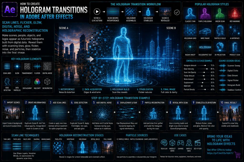
PART 11 — HOLOGRAPHIC REVEAL

A holographic transition usually combines:

scan lines.

transparent color.

flicker.

noise.

Glow.

digital grid.

Step 12: Tint Scene B

Before it becomes fully normal:

apply cyan or blue tint.

Step 13: Reduce Opacity

Initially make Scene B:

semi-transparent.

Step 14: Add Scan Lines

Overlay thin horizontal lines.

Step 15: Add Glow

Highlight edges.

Step 16: Restore Normal Image

As reconstruction completes:

remove tint.

remove transparency.

reduce scan lines.

Scene B becomes fully solid.

Project 6 — Holographic Reconstruction

Scene B begins as transparent cyan hologram.

scan passes.

details appear.

color returns.

image becomes fully real.

PART 12 — FIND EDGES RECONSTRUCTION

A strong effect is to reveal Scene B in stages.

First:

outline.

Then:

wireframe-like appearance.

Then:

full image.

Step 17: Duplicate Scene B

Create:

SCENE_B_EDGES

Apply:

Find Edges.

Step 18: Invert or Tint

Use:

Invert.

Tint.

Glow.

Create bright cyan or white outlines.

Step 19: Reveal Edges Before Full Image

Scan line passes.

edge version appears first.

full Scene B follows several frames later.

Project 7 — Blueprint Scan Reveal

Scene A.

scan line passes.

wireframe edges appear.

full-color Scene B follows.

This works extremely well for:

architecture.

products.

technology.

maps.

PART 13 — MULTI-STAGE RECONSTRUCTION

Use four stages:

Stage 1 — Noise

Stage 2 — Grid

Stage 3 — Edge Detection

Stage 4 — Full Image

As the scanner passes:

noise becomes structure.

structure becomes outline.

outline becomes image.

PART 14 — DATA PARTICLE RECONSTRUCTION

Create particles around the scanning edge.

You can use native particle tools.

Particles appear ahead of the line and disappear once the image stabilizes.

Step 20: Create Particle Layer

Create:

SCAN_PARTICLES

Use:

CC Particle World

or another suitable particle effect.

Step 21: Keep Particles Near Scan Boundary

Use a mask or position animation.

Step 22: Match Color

Use:

cyan.

green.

purple.

white.

Project 8 — Particle Data Scan

Small particles gather.

scan passes.

particles form image.

particles disappear.

Scene B becomes stable.

PART 15 — PIXEL RECONSTRUCTION

Combine the previous pixel-transition techniques.

Behind the scan line:

Scene B first appears as:

large Mosaic blocks.

Then:

pixel size decreases.

Finally:

image becomes sharp.

Step 23: Apply Mosaic to Scene B

Start behind scan line with large pixels.

Step 24: Reduce Pixel Size Over Time

Animate toward normal.

Project 9 — Pixel Scan Reveal

Scan line passes.

Scene B appears pixelated.

pixels become smaller.

image sharpens.

PART 16 — DATA COLUMN REVEAL

Instead of a continuous line:

use multiple thin columns.

Each column activates at a slightly different time.

This creates a digital reconstruction pattern.

PART 17 — DATA ROW REVEAL

Use horizontal strips.

Stagger them.

Scene B appears row by row.

PART 18 — VENETIAN BLINDS SCAN

Use:

Venetian Blinds.

Create thin repeating bands.

Animate completion.

This can simulate a scan-line reveal.

PART 19 — SCANLINE FLICKER

Create thin horizontal lines over the entire image.

Animate:

Opacity.

Position.

Random flicker.

Keep subtle.

PART 20 — CRT-STYLE SCAN

For retro digital interfaces:

use:

scan lines.

green tint.

small noise.

slight distortion.

rounded-screen vignette.

Project 10 — Retro Computer Scan

Black screen.

green scan line.

image reconstructs.

text appears.

small signal noise.

PART 21 — AI SCAN STYLE

For AI-related visuals:

use:

cyan.

purple.

blue.

data particles.

bounding boxes.

labels.

transparent grids.

PART 22 — CYBERSECURITY SCAN

Use:

green or cyan.

target boxes.

network lines.

security labels.

digital noise.

PART 23 — FACE SCAN TRANSITION

Use a portrait.

Add:

horizontal scanner.

facial landmark points.

bounding boxes.

ID labels.

Then transition to another scene.

Project 11 — Biometric Scan Reveal

Face visible.

scanner travels downward.

facial grid appears.

data labels activate.

image transitions into digital profile or second shot.

PART 24 — PRODUCT SCAN

This is excellent for technology products.

Use:

phone.

laptop.

camera.

car.

appliance.

Step 25: Reveal Edges First

Use Find Edges.

Step 26: Add Measurement Lines

Create:

dimension indicators.

feature labels.

Step 27: Restore Full Product

As scan completes.

Project 12 — Product Analysis Transition

Product begins normal.

scan starts.

surface becomes wireframe.

feature callouts appear.

new product angle reconstructs.

PART 25 — BUILDING SCAN

For architecture:

reveal:

wireframe.

structural grid.

full render.

This works for:

real estate.

architecture.

construction.

PART 26 — MAP SCAN TRANSITION

Scan across a map.

Behind the scanner:

new geographic layer appears.

Examples:

satellite → terrain.

terrain → data map.

map → route network.

Project 13 — Map Data Reconstruction

Flat map.

scan line crosses.

roads activate.

location markers appear.

data network emerges.

PART 27 — TERRAIN SCAN

Combine with the 3D terrain series.

A scanner can move across terrain and reveal:

elevation.

contour lines.

temperature.

network data.

mineral zones.

PART 28 — MEDICAL-STYLE SCAN

For generic fictional visualization:

use:

slice scanning.

cross sections.

grids.

anatomical imagery only where appropriate.

PART 29 — LASER SWEEP

A laser-style scan can be much brighter than a normal line.

Create:

bright line.

strong Glow.

lens flare if appropriate.

Step 28: Add Light Falloff

Create soft gradient above and below the line.

Step 29: Add Bloom

Use Glow.

Project 14 — Laser Reconstruction

Dark object.

laser moves across.

surface details appear.

object becomes illuminated.

new scene forms.

PART 30 — MULTIPLE LASER LINES

Use:

parallel beams.

Offset slightly in time.

This creates a scanning-array effect.

PART 31 — SCANNER LIGHT BAR

Create thick bright band.

Use:

gradient.

soft edges.

Scene B becomes visible beneath.

This resembles:

photocopier.

document scanner.

machine-vision device.

PART 32 — CAMERA SCAN FLASH

A Camera-style bright scan can momentarily overexpose part of the frame.

Use:

Exposure.

Glow.

moving gradient.

PART 33 — HOLOGRAPHIC FLICKER

Before Scene B stabilizes:

flicker Opacity.

For example:

100%.

30%.

80%.

0%.

100%.

Keep timing brief.

PART 34 — HOLOGRAM DISTORTION

Apply:

Displacement Map.

Use:

horizontal noise.

Animate slightly.

The hologram becomes unstable.

PART 35 — HOLOGRAPHIC COLOR SEPARATION

Add subtle RGB or cyan/magenta separation.

Keep smaller than a full glitch effect.

PART 36 — HOLOGRAM TRANSPARENCY

Blend Scene B with the background.

Use:

Screen.

Add.

or reduced Normal Opacity.

Restore to solid later.

PART 37 — GRID PROJECTION

Create a grid that appears to project into 3D space.

Use:

3D Layer.

Camera.

Perspective.

Project 15 — 3D Hologram Reconstruction

Ground plane.

grid appears.

particles rise.

wireframe forms.

full object appears.

PART 38 — SCAN THROUGH 3D SPACE

Enable the scan line or plane as a 3D layer.

Move it through:

Z space.

Rather than simply across the screen.

PART 39 — VOLUMETRIC SCAN PLANE

Create a semi-transparent rectangle.

Give it:

Glow.

gradient.

noise.

Move through a 3D model or layered composition.

PART 40 — CAMERA FLY-THROUGH SCAN

Camera moves toward a digital scan plane.

Pass through it.

Scene changes on the other side.

This creates a seamless environment transition.

Project 16 — Scan Portal

Scene A.

digital scan plane ahead.

Camera approaches.

plane fills frame.

cut.

Camera emerges into Scene B.

PART 41 — OBJECT-BASED SCAN TRANSITION

Use an object already in the scene.

Examples:

doorway.

screen.

glass panel.

window.

scanner frame.

The scan originates from that object.

PART 42 — SCREEN SCAN TRANSITION

Display scanning line on:

phone.

monitor.

tablet.

Then zoom into the screen.

Scene B takes over.

PART 43 — BARCODE-STYLE SCAN

Create vertical bars.

Move a laser line across.

New scene appears as bars decode.

Useful for:

retail.

logistics.

inventory.

technology.

PART 44 — QR-STYLE RECONSTRUCTION

Build a square-cell pattern.

Progressively replace it with Scene B.

Use for visual style rather than necessarily encoding real data.

PART 45 — DATA PARTICLE STREAM

Particles can flow into the image rather than simply appearing.

Use:

streams.

trails.

data points.

PART 46 — PARTICLE ASSEMBLY

Scene B appears to form from thousands of dots.

Keep particles concentrated near the scan boundary.

PART 47 — EDGE PARTICLES

Emit particles from the transition edge.

As the scanner passes:

particles travel briefly.

fade.

PART 48 — GRID DEFORMATION

Distort grid slightly using:

Displacement Map.

Fractal Noise.

This creates a more advanced sci-fi look.

PART 49 — LIGHT SWEEP

Use:

CC Light Sweep

where appropriate.

Animate across:

text.

logo.

product.

This can reinforce the scanner.

PART 50 — ADDING LABELS

Add digital labels such as:

SCANNING.

ANALYZING.

PROCESSING.

COMPLETE.

Example Sequence

SCANNING… 23%

SCANNING… 67%

RECONSTRUCTION COMPLETE

Use only when it suits the design.

PART 51 — PROGRESS BAR

Create a simple horizontal bar.

Link it to scanner progress.

For example:

0% → 100%.

PART 52 — PERCENTAGE COUNTER

Create:

0%.

25%.

50%.

75%.

100%.

Animate alongside scan.

PART 53 — HUD ELEMENTS

Add:

corners.

crosshairs.

targets.

coordinate labels.

data readouts.

Keep them subordinate to the main transition.

PART 54 — SCANNER CROSSHAIR

A moving crosshair can follow the scan line or important object.

PART 55 — DATA POINT ACTIVATION

As scan passes:

small nodes appear.

This works especially well for:

maps.

products.

faces.

technology.

PART 56 — COLOR TRANSITION

Scene A and Scene B may have different colors.

Use the scan boundary to manage the change.

Ahead of scan:

Scene A grade.

Behind:

Scene B grade.

PART 57 — EXPOSURE TRANSITION

Same idea with brightness.

The scan can literally appear to relight the image.

Project 17 — Day-to-Night Scan

Daytime city.

scan line crosses.

behind scanner:

night city appears.

building lights activate.

This creates a strong before-and-after effect.

PART 58 — BEFORE-AND-AFTER REVEAL

Use scanner to compare:

raw footage → color grade.

before → after.

old design → new design.

wireframe → final render.

PART 59 — PRODUCT COLOR CHANGE

Scan across product.

Behind:

different color or material appears.

PART 60 — DAMAGE REPAIR EFFECT

Scan across damaged image or object.

Behind:

clean version appears.

Useful for:

restoration.

repair.

before-and-after visualization.

PART 61 — BLUEPRINT TO REALITY

This is one of the best scan-transition applications.

Scene A:

blueprint.

scanner moves.

Scene B:

finished building.

Project 18 — Blueprint Reconstruction

Architectural drawing.

scanner crosses.

wireframe appears.

textures develop.

completed building fills frame.

PART 62 — SKETCH TO PHOTO

Same technique.

Scene A:

drawing.

Scene B:

real photograph.

PART 63 — MAP TO SATELLITE

Scene A:

graphic map.

scan.

Scene B:

satellite imagery.

PART 64 — TERRAIN TO DATA

Scene A:

mountains.

scan.

Scene B:

contour lines, data nodes, statistics.

PART 65 — MASTER SCAN CONTROLLER

Create:

SCAN_CTRL

Add:

Scan Progress.

Line Brightness.

Glow Amount.

Noise Strength.

Pixel Size.

Hologram Opacity.

Grid Opacity.

Distortion.

PART 66 — LINK PROGRESS TO POSITION

Use:

Scan Progress:

0–100%.

Map it to:

line Position.

matte Position.

progress bar.

data percentage.

PART 67 — LINK RECONSTRUCTION TO PROGRESS

Behind the scanner:

Mosaic decreases.

hologram becomes opaque.

color returns.

grid disappears.

PART 68 — SCAN SPEED

Not every scan should move linearly.

Use:

slow start.

steady middle.

small slowdown at important object.

fast finish.

PART 69 — GRAPH EDITOR

Use Easy Ease and Graph Editor for:

scan-line movement.

Camera motion.

large opacity changes.

PART 70 — HOLD KEYFRAMES

Use Hold keyframes for:

digital flickers.

data labels.

noise bursts.

status changes.

PART 71 — SCANNER TRAILING DELAY

The full-color Scene B does not need to appear exactly at the scanning line.

A polished setup might use:

scan line.

then 3 frames later:

wireframe.

then 4 frames later:

full image.

This creates layered reconstruction.

PART 72 — DISTORTION AHEAD OF SCANNER

Add small displacement just before the scan line reaches an area.

This creates anticipation.

PART 73 — STABILIZATION BEHIND SCANNER

Keep tiny flicker or noise for several frames after the scan passes.

Then stabilize.

PART 74 — SCAN SOUND DESIGN

Sound is critical.

Useful sounds include:

laser sweeps.

electronic hum.

data ticks.

digital beeps.

scanner motors.

electrical pulses.

holographic whooshes.

Scan Sound Structure

Start:

quiet electronic hum.

Movement:

rising scanner sweep.

During reconstruction:

data clicks.

Completion:

short confirmation tone.

PART 75 — PROGRESS BEEPS

Use small digital ticks as percentage increases.

Avoid excessive repetition.

PART 76 — LOW-FREQUENCY HUM

A subtle underlying hum can make the effect feel more physical.

PART 77 — COMPLETION SOUND

At 100%:

use a restrained:

beep.

click.

impact.

confirmation tone.

PART 78 — AUDIO BRIDGE

Begin Scene B ambience before reconstruction finishes.

This helps make the scene transition feel continuous.

PART 79 — TRANSITION DURATION

Typical timings:

8–15 frames: fast scan wipe.

15–30 frames: standard digital transition.

1–2 seconds: detailed holographic reconstruction.

2–4 seconds: cinematic analysis scan.

PART 80 — PERFORMANCE

Glow, particles, noise, displacement, and grids can slow previews.

During editing:

disable expensive Glow.

reduce preview resolution.

disable particles.

re-enable for final review.

Build Reusable Scan Presets

Create:

CLEAN SCAN

LASER SCAN

HOLOGRAM

PIXEL REBUILD

RADAR SCAN

GRID REVEAL

BIOMETRIC SCAN

BLUEPRINT RECONSTRUCTION

Recommended Project Organization

Create folders:

SCENE_A

SCENE_B

SCAN_MATTES

SCAN_LINES

GRID

HOLOGRAM

PARTICLES

HUD

AUDIO

CONTROLS

Suggested Layer Stack

HUD_ELEMENTS

SCAN_PARTICLES

SCAN_LINE

SCAN_GLOW

SCENE_B_FULL

SCENE_B_EDGES

SCENE_B_PIXEL

SCAN_MATTE

SCENE_A

SCAN_CTRL

AUDIO

Common Mistake: Scan Line and Reveal Don’t Match

The boundary must remain synchronized.

Common Mistake: Too Much Glow

Keep the core line visible.

Common Mistake: Every Effect Is Cyan

Use cyan deliberately, not automatically.

Other strong palettes include:

green.

purple.

orange.

white.

red.

Common Mistake: Scene B Becomes Full Quality Instantly

Use staged reconstruction.

Common Mistake: Grid Is Too Strong

Keep it subtle.

Common Mistake: Scan Moves Too Fast to Read

Allow enough time for viewers to understand the mechanism.

Common Mistake: Particle Count Is Excessive

Particles should support the reconstruction rather than obscure it.

Common Mistake: No Trailing Effects

Add slight delay between scanner, wireframe, and full image.

Common Mistake: Interface Elements Cover the Scene

HUD graphics should remain secondary.

Common Mistake: No Sound

Scanner audio adds substantial credibility.

Basic Digital Scan Transition Quick Recipe

1. Import Scene A.
2. Import Scene B.
3. Create Scan Matte.
4. Animate matte across frame.
5. Create glowing Scan Line.
6. Match line to matte.
7. Add trailing Glow.
8. Create Scene B edge version.
9. Create Scene B pixel version.
10. Reveal edge version first.
11. Reveal pixel version.
12. Reveal full image.
13. Add grid.
14. Add particles.
15. Add noise.
16. Add small displacement.
17. Add HUD elements.
18. Add scanner sound.
19. Preview.
20. Refine.

Clean Scan Recipe

Use:

one line.

Glow.

simple matte.

minimal interface graphics.

Holographic Scan Recipe

Use:

cyan tint.

edge detection.

scan lines.

particles.

transparency.

flicker.

Pixel Reconstruction Recipe

Use:

Mosaic.

scan matte.

progressive pixel reduction.

Laser Scan Recipe

Use:

bright line.

strong Glow.

light falloff.

electronic sweep.

Radar Recipe

Use:

rotating wedge.

circular grid.

location markers.

Blueprint Recipe

Use:

Find Edges.

blue/cyan tint.

grid.

full-render reveal.

Five Essential Scan Exercises

Exercise 1 — Horizontal Scan

Learn the matte and scan-line relationship.

Exercise 2 — Edge Reconstruction

Reveal a wireframe-style image before the full scene.

Exercise 3 — Pixel Reconstruction

Combine scan movement with Mosaic.

Exercise 4 — Holographic Scan

Add transparency, grid, Glow, and flicker.

Exercise 5 — Blueprint-to-Reality Transition

Combine multiple reconstruction stages into one polished sequence.

Master these five exercises and you’ll understand the core techniques behind digital scanning transitions.

Frequently Asked Questions

How do I create a digital scan transition in After Effects?

Use an animated matte to reveal the next scene, place a glowing scan line on the matte boundary, and add digital reconstruction effects behind it.

Can I create the effect without plug-ins?

Yes.

The core workflow can be built with native After Effects effects and Shape Layers.

How do I create the scanning line?

Use a Shape Layer Stroke with Glow and animate its Position.

Can I reveal Scene B as a hologram first?

Yes.

Tint it, reduce Opacity, add scan lines, edge detection, noise, and Glow before restoring the normal image.

How do I create a wireframe look?

Find Edges combined with Tint, Invert, and Glow can create a stylized outline.

Can I reconstruct the image from pixels?

Yes.

Use Mosaic and progressively reduce pixel size behind the scan line.

Can I add particles?

Yes.

Particles can gather near the scanner or appear as the scene reconstructs.

Can I make a radial scan?

Yes.

Use an expanding circle or rotating radar wedge instead of a linear matte.

Can I use this for products?

Yes.

Product scanning is one of the strongest applications of the effect.

Can I use it for maps?

Yes.

Scanning can reveal roads, routes, data layers, terrain, or satellite imagery.

Can I use it for architecture?

Yes.

Blueprint-to-building reconstruction works particularly well.

Do I need third-party plug-ins?

No.

Practice Project: Holographic City Reconstruction

Create:

DIGITAL_SCAN_MASTER

at:

1920 × 1080.

Import:

SCENE_A — Dark Digital Grid

SCENE_B — Futuristic City

Create:

SCAN_MATTE

Animate:

top → bottom.

Create:

SCAN_LINE

Use:

cyan Stroke.

Add:

Glow.

Create:

SCENE_B_PIXEL

Apply:

Mosaic.

Create:

SCENE_B_EDGES

Apply:

Find Edges.

Tint:

cyan.

Add:

Glow.

Create:

SCENE_B_FULL

normal footage.

As the scanner moves:

first reveal:

pixel version.

Several frames later:

edge version.

Then:

full image.

Add:

SCAN_GRID.

Add:

small data particles near the boundary.

Add:

horizontal Noise.

Apply:

subtle Displacement Map near scan line.

Create:

HUD text:

SCANNING

Then:

RECONSTRUCTING

Then:

COMPLETE

Add progress counter:

0% → 100%.

Sound design:

low electronic hum.

scanner sweep.

small digital clicks.

short completion tone.

Begin city ambience before the final image fully stabilizes.

The viewer should experience:

dark digital environment.

scanner activates.

pixels appear.

city edges reconstruct.

detail fills in.

full futuristic city becomes visible.

interface confirms completion.

That one project teaches:

animated mattes,

scan lines,

Glow,

edge detection,

Mosaic reconstruction,

particles,

HUD graphics,

displacement,

and:

sound design.

If you’d like to create these effects yourself, you can explore Adobe’s current After Effects options below:

Get Adobe After Effects and start creating digital scan transitions, holographic reveals, laser sweeps, HUD effects, and data reconstruction animations

What Should You Learn Next?

After digital scan transitions, the next strong futuristic technique is the hologram transition.

We’ll take the scanner concept further and make entire people, objects, products, and environments appear as unstable holographic projections before becoming fully solid.

We’ll cover:

scan lines.

transparency.

RGB separation.

digital noise.

flicker.

Glow.

displacement.

particle reconstruction.

The next article will therefore be:

How to Create Hologram Transitions in Adobe After Effects: Scan Lines, Flicker, Glow, Digital Noise, and Holographic Reconstruction.

Final Thoughts

Digital scan transitions are built around one simple idea:

the next scene is generated progressively rather than simply appearing.

The scan line gives the viewer a clear visual cause.

Behind that line, the image changes state:

pixels appear.

edges form.

data points activate.

color returns.

the scene becomes complete.

The strongest results use several reconstruction stages instead of one immediate reveal.

Start with the matte.

Keep the scanner synchronized.

Then layer in:

Glow.

grid.

pixelation.

edge detection.

particles.

noise.

HUD elements.

sound.

Once those elements work together, the transition can feel like a futuristic imaging system rather than a conventional wipe.

Explore Adobe After Effects and start creating professional digital scan and holographic transition effects